Figure Analysis (Windows)🪶

Figure 1 - Training Curves🪶

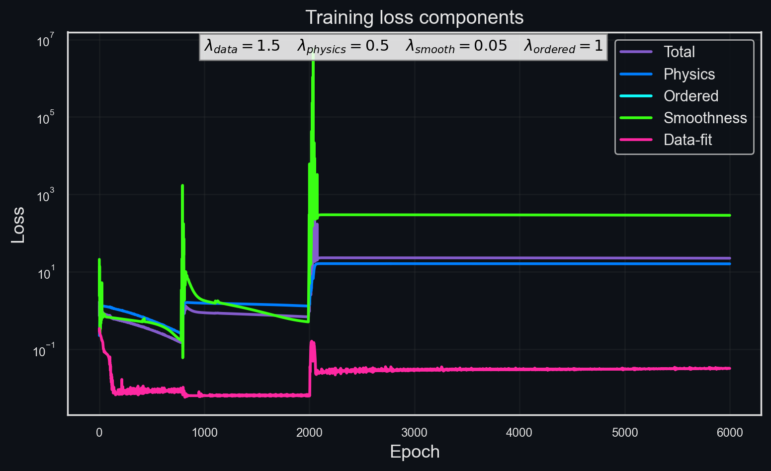
Figure 1 Analysis

Take-Home Message

The optimizer exhibits three distinct regime transitions before settling on a stable plateau.

🔑 Key Insights

Spike 1 ($\approx$ 0-50 epochs) - Expected transient while the network adjusts from random initial weights.
Spike 2 ($\approx$ 800 epochs) - Discovery of a higher-curvature potential: smoothness and total loss spike, physics and data terms rise only moderately.
Spike 3 ($\approx$ 2000 epochs) - Order-of-magnitude jump in the smootheness term propagates into the physics loss; a new plateau follows with lower smothness fidelity, but improved data fit.

❌ Failure Modes

Verdict	Failure Mode	Description	Explanation
❌	High final loss	Optimizer stalls in a local minimum.	Total loss remains greater than 1e-1 at epoch 6000.
✔️	Oscillation avoided	Unbalanced loss weights can cause loss terms to oscillate.	Curves converge monotonically after Spike 3.
❌	Physics collapse	Data loss decreases, while TISE residual increases.	Indicates operator inconsistency.
❌	Over-regularization	Smoothness term dominates, spectrum becomes innacurate.	Post-Spike 3 plateau shows $\lambda_\text{smooth}$ is much greater than others.

Sanity Checks🪶

Figure 2 - $V_\theta$ vs. $V(x)$🪶

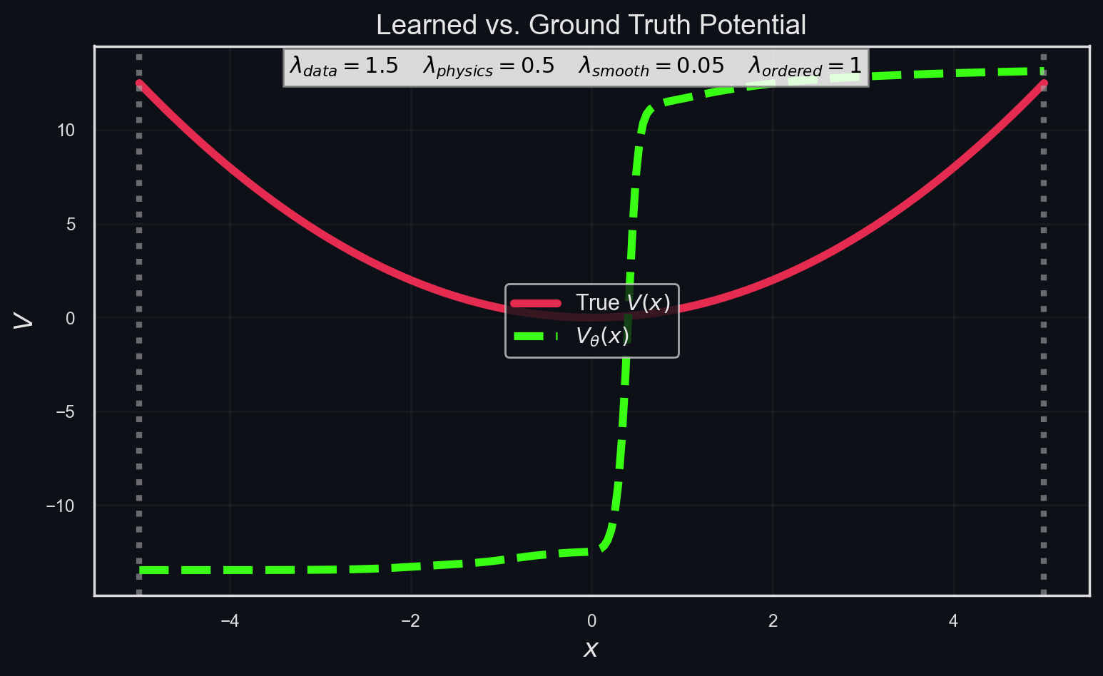
Figure 2 Analysis

Take-Home Message

The learned potential $V_\theta(x)$ (sigmoidal) differs markedly from the harmonic ground truth $V(x)=\tfrac12 x^2$.

🔑 Key Insights

Central regions of the learned eigenfunctions (Fig. 3) and densities (Fig. 5) match the ground truth far better than the tails.
The model learns only the portion of $H_\theta$ required to reproduce high-probability regions, exposing the inverse problem's under-determinism.

❌ Failure Modes

Verdict	Failure Mode	Description	Explanation
❌	Gemoetric mismatch	Learned $V_\theta$ shape incompatible with true quadratic.	Central well too narrow; tails saturate at $V_\theta \approx \pm 12 $.
❌	Boundary under-constraint	Sparse data at $x \in (-\infty, -4.5] \cup [4.5, \infty)$ allows the potential to drift.	Grey dashed domain limits show no training points beyond.

Figure 3 – $\{\psi_n^\theta\}$ vs. $\{\psi_n\}$🪶

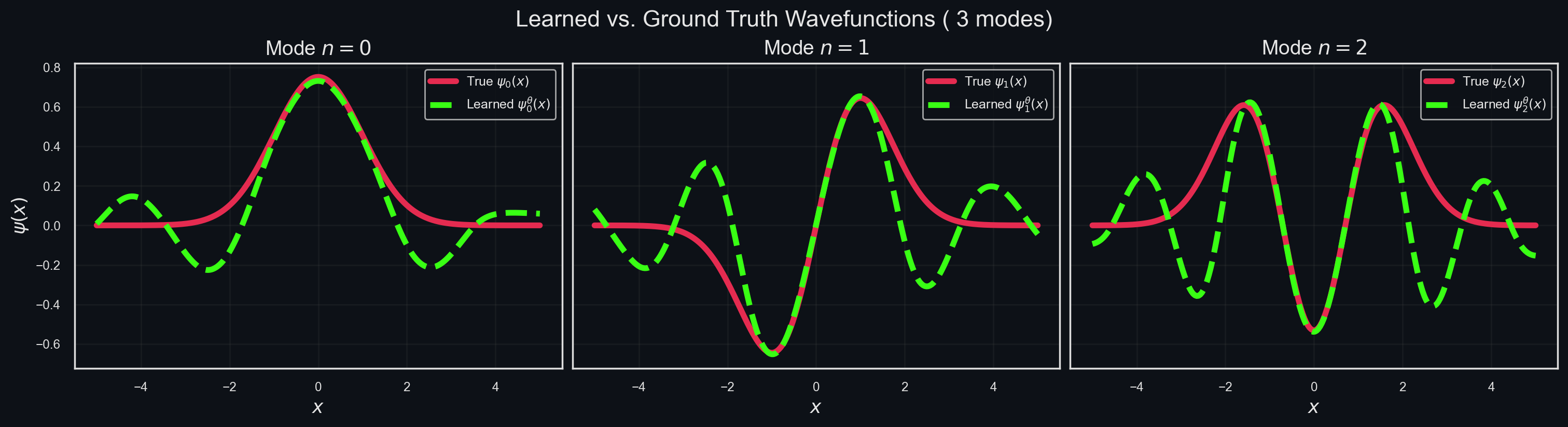
Figure 3 Analysis

Take-Home Message

Learned eigenfunctions $\psi_n^\theta(x)$ capture the nodal pattern but diverge in low-amplitude tail regions.

🔑 Key Insights

Phase matching - Correct nodal count confirms energy ordering.
Central accuracy - Highest fidelity occurs where $|\psi_n|^2$ is largest.
Tail divergence - For $x \in (-4.5, -2] \cup [2, 4.5)$, the learned curves overshoot, reflecting data scarcity.

❌ Failure Modes

Verdict	Failure Mode	Description	Explanation
❌	Nodal mis-count	Extra nodes appear beyond $x \approx \pm 3$)	Indicates spectral leakage.
✔️	Sign / parity flip	Unaligned solutions may invert parity	Sign aligned; parity matches ground truth.
❌	Spurious oscillations	High-frequency ripples in tails from weak $V_\theta$ smoothness.	Visible beyond $x\approx \pm 4$.

Figure 4 – $\{E_n^\theta\}$ vs. $\{E_n\}$🪶

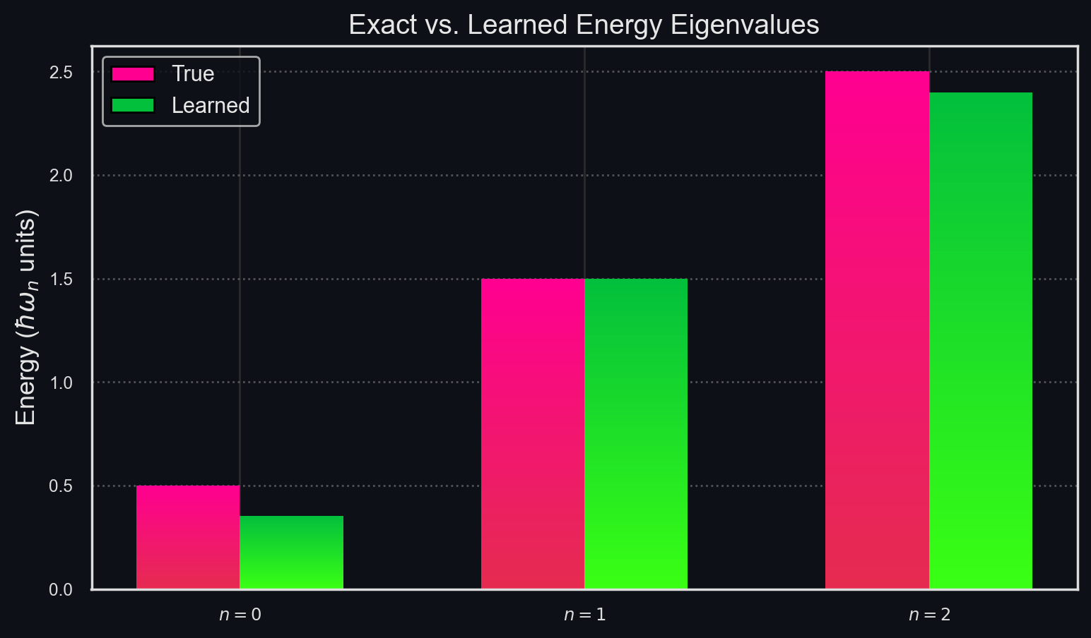
Figure 4 Analysis

Take-Home Message

Learned energies $E_n^\theta$ follow the harmonic spectrum $E_n=n+\tfrac12$ and match observations within 5 %.

🔑 Key Insights

Correct ordering suggests $\mathcal{L}_\text{order}$ is effective.
Spectrum remains stable despite 2z% Gaussian noise in training data.

❌ Failure Modes

Verdict	Failure Mode	Description	Explanation
❌	Spectral fit, wrong operator	Energies match, but $V_\theta$ deviates (see Fig. 2)

Figure 5 - $\{|\psi_n^\theta|^2\}$ vs.$\{\rho_n^\text{observed}\}$🪶

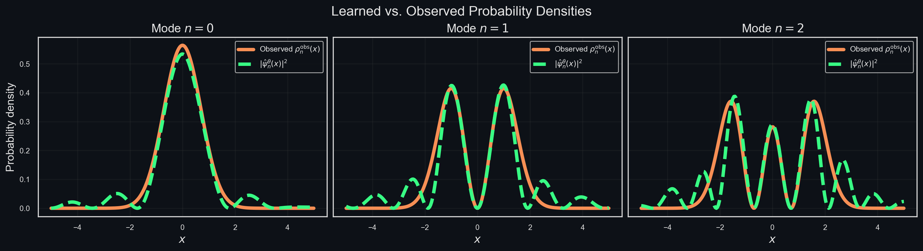
Figure 5 Analysis

Take-Home Message

Learned densities, $\rho_n^\theta = |\psi_n^\theta|^2$ agree with 2%-noise observations.

🔑 Key Insights

Noise filtering - PINN acts as a physics-informed smoother.
Data dominance - Good density fit persists even with incorrect potential (Fig. 2), confirming $\mathcal{L}_\text{data}$ is easy to minimize.

❌ Failure Modes

Verdict	Failure Mode	Description	Explanation
✔️	Peak flattening	Excessive $\lambda_\text{smooth}$ can lower peaks	Peaks are preserved $\Rightarrow$ smoothing is well-tuned.
✔️	Mode merging	Energy mis-ordering can collapse multiple states onto one density.

POD Analysis🪶

Figure 6 - POD Singular Values🪶

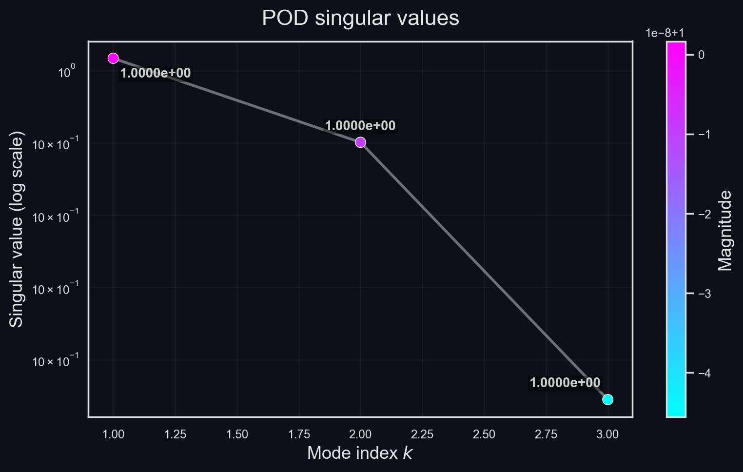
Figure 6 Analysis

Take-Home Message

Singular values from the POD of the learned wavefunction matrix decrease (log scale) from $\approx 1$.

🔑 Key Insights

Rank efficiency - Rapid two-decade decay indicates a low-dimensional basis.
Basis conditioning - Separation between $\sigma_0$, $\sigma_1$, and $\sigma_2$ quantifies how much "physics" each node carries.

❌ Failure Modes

Verdict	Failure Mode	Description	Explanation
❌	Flat spectrum	All $\sigma_i$ nearly equal $\Rightarrow$ modes are independent, but unphysical.	Would signal noise-dominated snapshots (❓).
❌	Slow decay	$\tfrac{\sigma_{2}}{\sigma_{0}} \geq 0.3 \Rightarrow$ redundant or correlated modes.	Implies over-fitting or aliasing in $\hat{\psi}_n^\theta$.

Figure 7 - Overlap matrix $\langle \hat{\psi}_m^\theta | \hat{\psi}_n^\theta \rangle $🪶

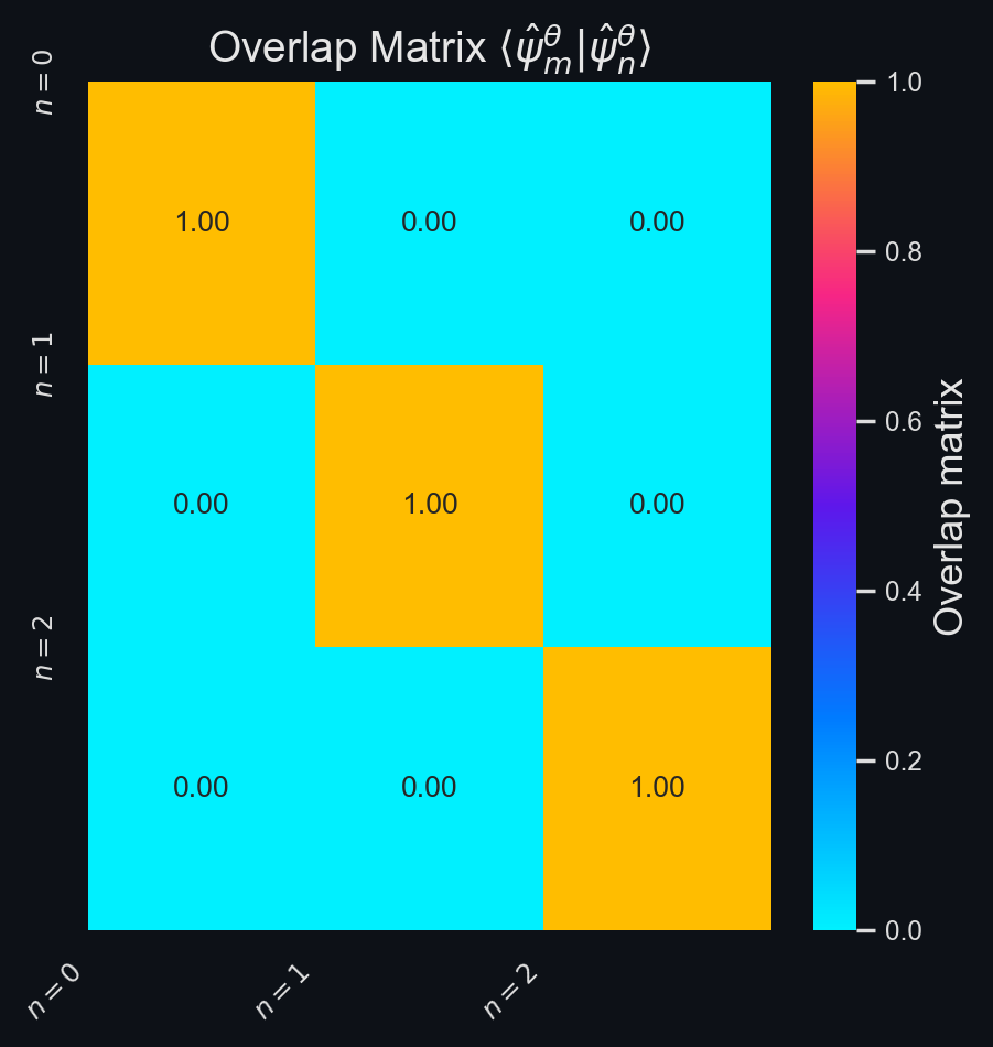
Figure 7 Analysis

Take-Home Message

Overlap matrix $\langle \hat{\psi}_i^\theta | \hat{\psi}_j^\theta \rangle$ confirms orthogonality of learned eigenfunctions.

🔑 Key Insights

Orthogonality: - Diagonals are $\approx 1$, off-diagonals are $\approx 0$ confirms Hermitian structure.
Basis consistency - Any bright off-diagonal would expose weak $\mathcal{L}_\text{physics}$.

❌ Failure Modes

Verdict	Failure Mode	Description	Explanation
✔️	Non-orthogonality	Off-diagonal $> 0.1$ indicates incomplete convergence	Here, max off-diagonal is $\ge 0.02$ $\Rightarrow$ passes.

Figure 8 - $\{u_n\}$ vs. $\{\hat{\psi}_n^\theta\}$ vs. $\{\hat{\psi}_n\}$🪶

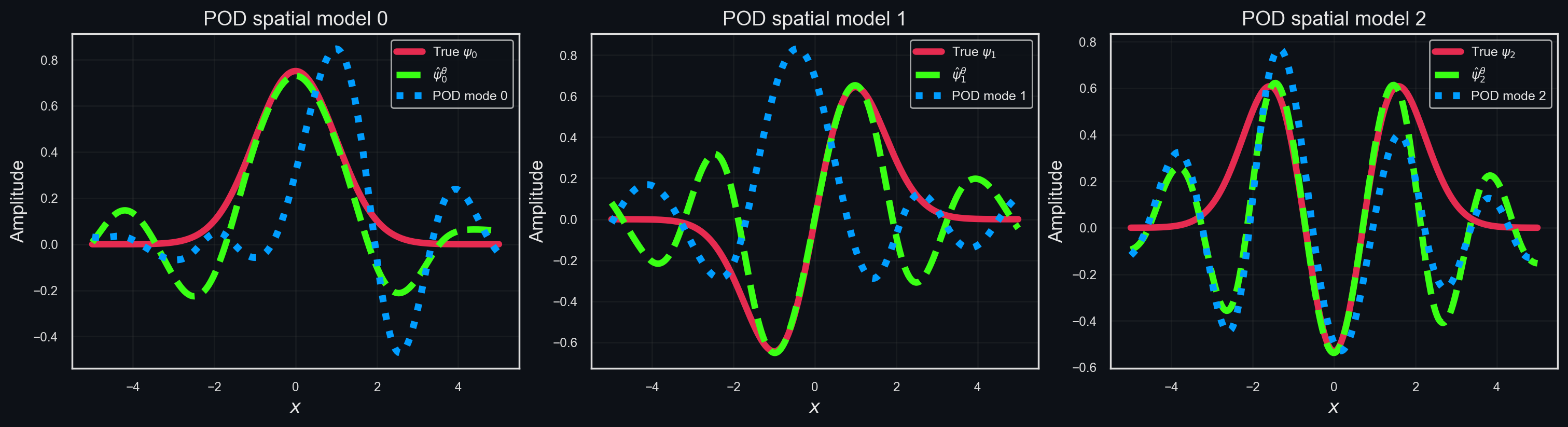
Figure 8 Analysis

Take-Home Message

First three POD modes (blue) compared with learned $\hat{\psi}_i^\theta$ (green) and ground truth $\hat{\psi}_i$ (red).

🔑 Key Insights

Geometric structure – Similarity to $\hat{\psi}_n$ indicates a stable, data-driven basis.
Feature extraction - POD isolates the most persistent spatial patterns.

❌ Failure Modes

Verdict	Failure Mode	Description	Explanation
❌	Mode mixing	Pod modes do not resemble any physical eigenfunction.	Blue curves visibly shifted (see Sec. A.6); fix requires re-weighting.

Figure 9 - Overlap matrix $\langle u_k | \hat{\psi}_n^\theta \rangle$🪶

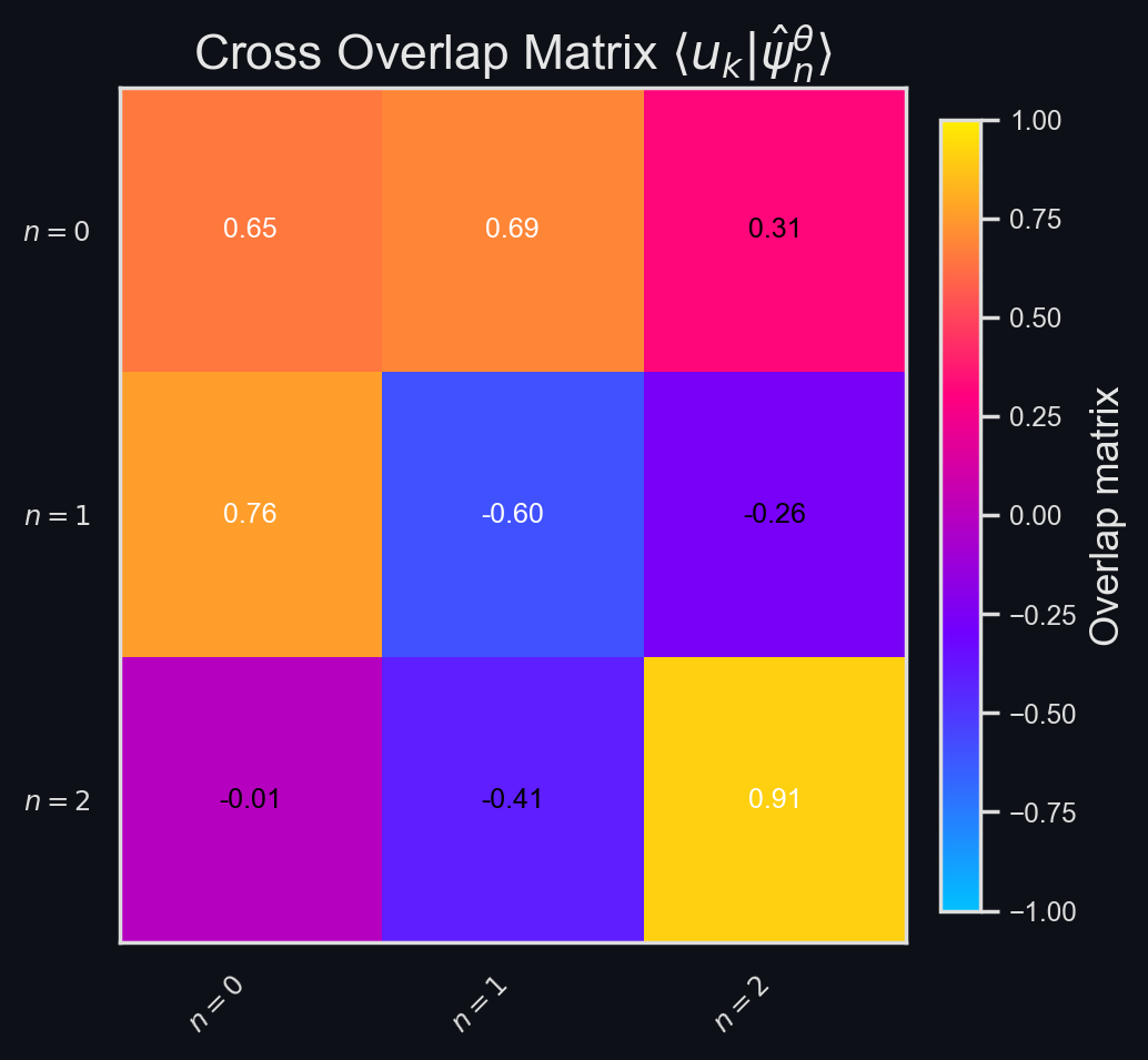
Figure 9 Analysis

Take-Home Message

Overlaps $\langle u_k | \hat{\psi}_n^\theta \rangle$ between POD spatial modes and learned wavefunctions.

🔑 Key Insights

Alignment - Ideal result is $\pm$ identity; here large off-diagonals show mis-alignment.
Energy concentration – Color magnitude reveals how energy distributes across modes.

❌ Failure Modes

Verdict	Failure Mode	Description	Explanation
❌	Distributed overlap	Single $u_k$ projects onto several $\hat{\psi}_n^\theta$.	🔮 Further investigation required to understand the root cause and impact on POD basis stability and interpretability.

Figure 10 - Overlap matrix $\langle u_k | \hat{\psi}_n \rangle$🪶

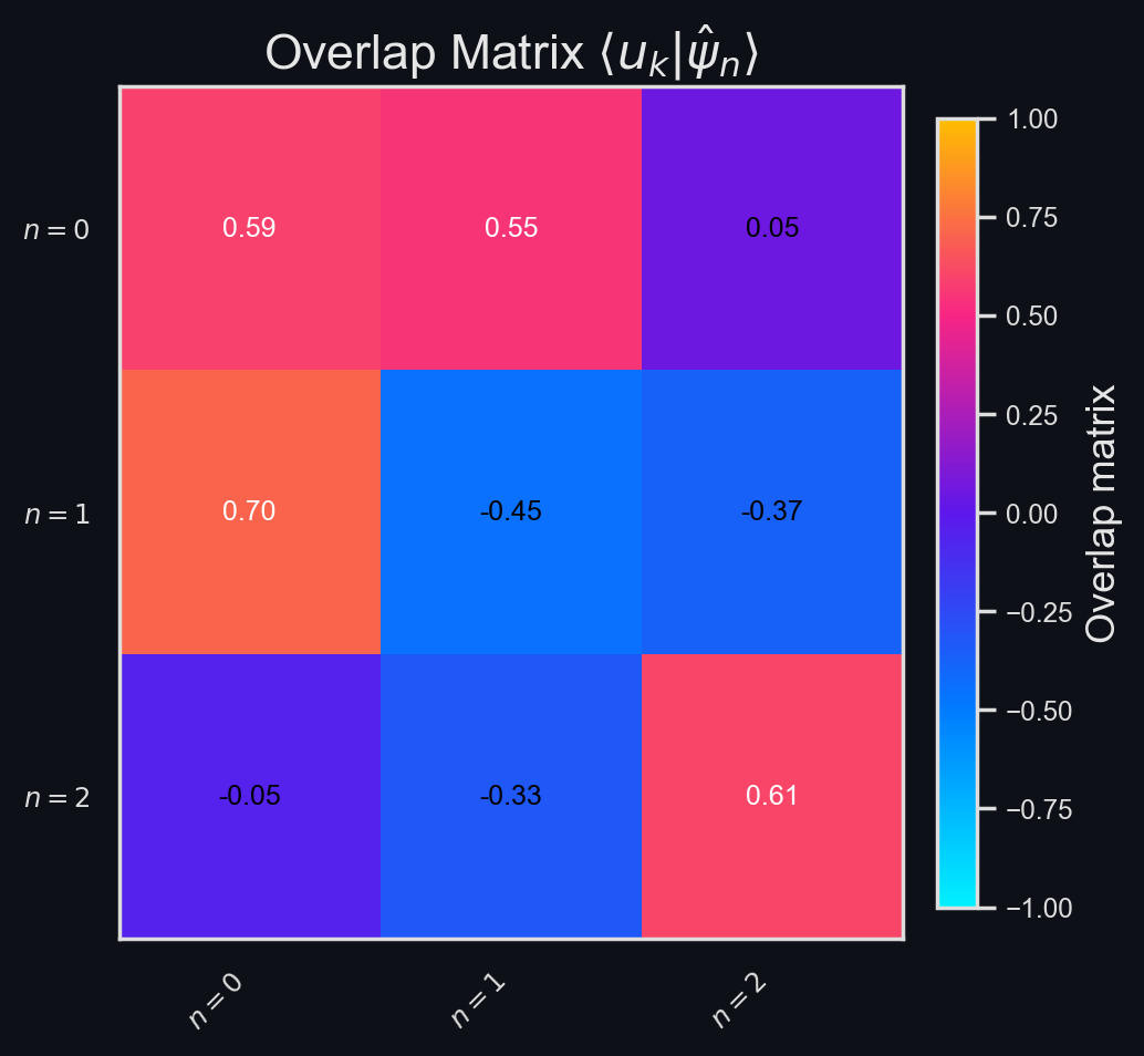
Figure 10 Analysis

Take-Home Message

Cross-overlap $\langle u_k | \hat{\psi}_n\rangle$ between physical POD modes and analytic ground-truth eigenfunctions.

🔑 Key Insights

Absolute consistency - High diagonal elements validate that the POD basis can recover the true physical basis.
Spectral recovery - Confirms operator structure even when $V_\theta$ differs.

❌ Failure Modes

Verdict	Failure Mode	Description	Explanation
❌	Mis-alignment	Off-diagonal $> 0.2$ indicates POD not yet physical	Here $\rangle u_0, \hat{\psi}_1 \rangle \approx 0.3 \Rightarrow $ Fix via rescaling (see text).

Figure 11 - Temporal Modes🪶

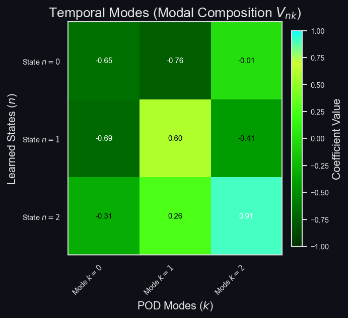
Figure 11 Analysis

Take-Home Message

Columns of $V$ from $\Psi=U\Sigma V^T$: modal composition per state.

🔑 Key Insights

Coefficient distribution - Shows how each POD mode contributes to each learned state.

❌ Failure Modes

Verdict	Failure Mode	Description	Explanation
❌	Incoherent coefficients	Random sign / magnitude pattern across rows of $V$.	Magnitudes scatter (cf. Fig. 13) $\Rightarrow$ indicates prior mis-alignment.

Figure 12 - Overlap Matrix $\langle v_m | v_n \rangle$🪶

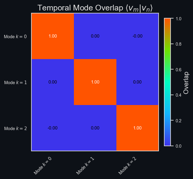
Figure 12 Analysis

Take-Home Message

Overlap $\langle v_m | v_n \rangle \approx I$, as expected.

🔑 Key Insights

Unitary property - Diagonals $\approx 1$, off-diagonals $\approx 0$ verifies numerical stability of SVD.

❌ Failure Modes

Verdict	Failure Mode	Description	Explanation
✔️	Identity deviation	Large off-diagonals	Largest off-diagonal $\approx 3\times 10^{-3} \Rightarrow$ within tolerance $\therefore$ pass.

Figure 13 - Overlap Matrix $|\langle \mathbf{e}_n | v_n \rangle|$🪶

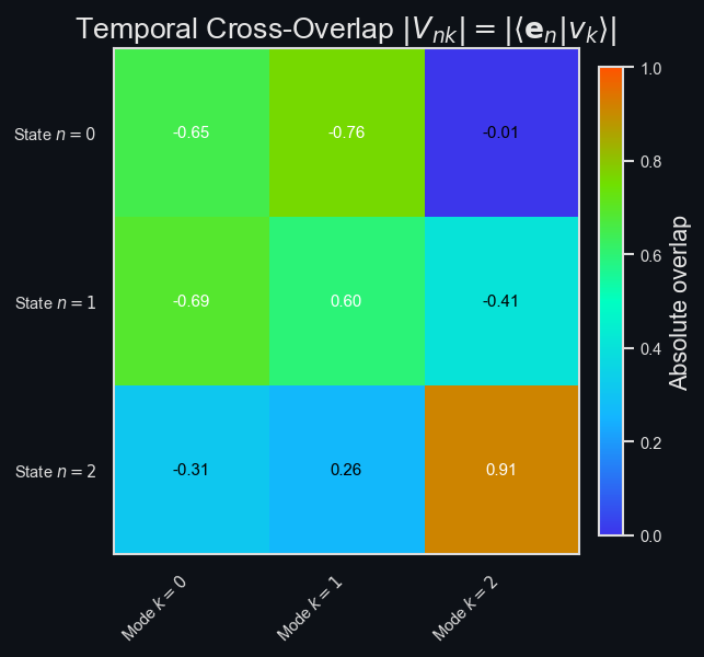
Figure 13 Analysis

Take-Home Message

Absolute coefficients $|V_{nk}| = |\langle \mathbf{e}_n | v_k \rangle|$ (basis vector vs. temporal mode).

🔑 Key Insights

Modal dominance - Ideally sparse with a bright diagonal; here large off-diagonals repeat the spatial misalignment story.

❌ Failure Modes

Verdict	Failure Mode	Description	Explanation
❌	Spread dominance	No clear diagonal; each state draws from several $v_k$.	Reflects same weighting bug; correcting $\psi_n^\theta$-scaling collapses to identity.

Figure Analysis (Windows)🪶

Figure 1 - Training Curves🪶

Sanity Checks🪶

Figure 2 - \(V_\theta\) vs. \(V(x)\)🪶

Figure 3 – \(\{\psi_n^\theta\}\) vs. \(\{\psi_n\}\)🪶

Figure 4 – \(\{E_n^\theta\}\) vs. \(\{E_n\}\)🪶

Figure 5 - \(\{|\psi_n^\theta|^2\}\) vs.\(\{\rho_n^\text{observed}\}\)🪶

POD Analysis🪶

Figure 6 - POD Singular Values🪶

Figure 7 - Overlap matrix $\langle \hat{\psi}_m^\theta | \hat{\psi}_n^\theta \rangle $🪶

Figure 8 - \(\{u_n\}\) vs. \(\{\hat{\psi}_n^\theta\}\) vs. \(\{\hat{\psi}_n\}\)🪶

Figure 9 - Overlap matrix \(\langle u_k | \hat{\psi}_n^\theta \rangle\)🪶

Figure 10 - Overlap matrix \(\langle u_k | \hat{\psi}_n \rangle\)🪶

Figure 11 - Temporal Modes🪶

Figure 12 - Overlap Matrix \(\langle v_m | v_n \rangle\)🪶

Figure 13 - Overlap Matrix \(|\langle \mathbf{e}_n | v_n \rangle|\)🪶

Verdict	Failure Mode	Description	Explanation
❌	Gemoetric mismatch	Learned \(V_\theta\) shape incompatible with true quadratic.	Central well too narrow; tails saturate at $V_\theta \approx \pm 12 $.
❌	Boundary under-constraint	Sparse data at \(x \in (-\infty, -4.5] \cup [4.5, \infty)\) allows the potential to drift.	Grey dashed domain limits show no training points beyond.

Verdict	Failure Mode	Description	Explanation
❌	Nodal mis-count	Extra nodes appear beyond \(x \approx \pm 3\))	Indicates spectral leakage.
✔️	Sign / parity flip	Unaligned solutions may invert parity	Sign aligned; parity matches ground truth.
❌	Spurious oscillations	High-frequency ripples in tails from weak \(V_\theta\) smoothness.	Visible beyond \(x\approx \pm 4\).

Verdict	Failure Mode	Description	Explanation
✔️	Peak flattening	Excessive \(\lambda_\text{smooth}\) can lower peaks	Peaks are preserved \(\Rightarrow\) smoothing is well-tuned.
✔️	Mode merging	Energy mis-ordering can collapse multiple states onto one density.

Verdict	Failure Mode	Description	Explanation
❌	Flat spectrum	All \(\sigma_i\) nearly equal \(\Rightarrow\) modes are independent, but unphysical.	Would signal noise-dominated snapshots (❓).
❌	Slow decay	\(\tfrac{\sigma_{2}}{\sigma_{0}} \geq 0.3 \Rightarrow\) redundant or correlated modes.	Implies over-fitting or aliasing in \(\hat{\psi}_n^\theta\).